






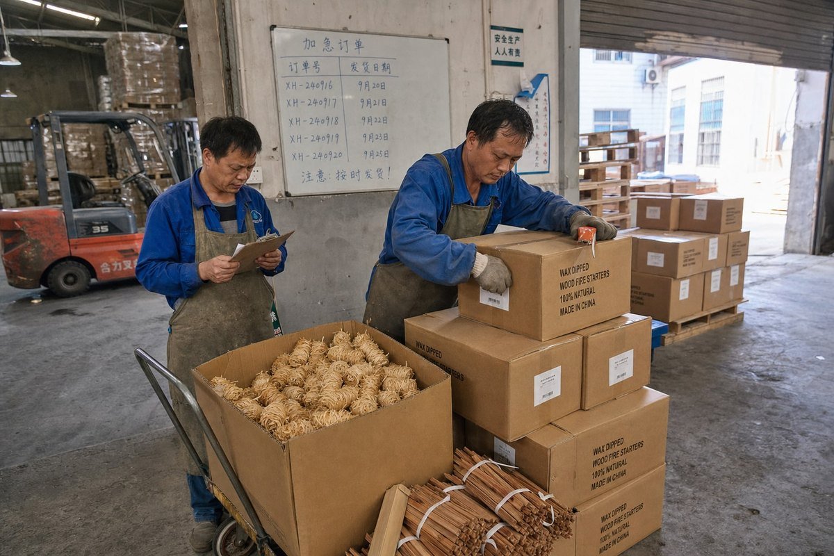
Every autumn, our production line in Ningbo fills with urgent wood fire starter orders from buyers who guessed wrong. Stockouts kill their season. Overstock kills their cash. There is a better way.
To forecast peak-season order quantities for wood fire starters, collect 2–3 years of clean monthly sales data, calculate seasonal indices, apply a year-over-year growth factor, add safety stock for lead time and demand variability, then subtract on-hand and in-transit inventory to get your purchase order quantity.
That formula sounds dense. So let me break it into four practical questions, in the order a purchasing manager would actually ask them.
What Sales Data Should I Collect to Build an Accurate Peak-Season Forecast?
A German distributor once showed me his forecast. It was last year's total plus 15%. He ran out of wax-dipped wood rolls by mid-November. His data was the problem, not his math.
Collect at least 24–36 months of monthly or weekly sales by SKU, cleaned of stockout periods, one-off promotions, and discontinued bundles. Then divide annual sales by 12 for a baseline, and divide each month's average by that baseline to build seasonal indices.

Wood fire starters are strongly seasonal. Demand climbs when heating season starts, and many markets show a second bump during summer grilling and camping. That dual-peak pattern is exactly why a flat average fails. In our experience exporting to the US, Germany, and the UK, buyers who track heating degree days 1 alongside their sales history spot the winter surge weeks earlier than buyers who only watch order totals.
Start with clean history
Dirty data produces confident but wrong forecasts. Before you calculate anything, fix these issues:
- Remove weeks where you were out of stock. Zero sales during a stockout is not zero demand.
- Flag one-time promotional spikes. A flash sale is not organic seasonal demand.
- Exclude discontinued SKUs and holiday gift bundles that will not repeat.
- Use continuous data with no large gaps.
Build the seasonal index
Here is the core method, using a simplified fictional SKU:
| Month | Avg. Units (3-yr) | Baseline (Annual ÷ 12) | Seasonal Index |
|---|---|---|---|
| July | 600 | 1,000 | 0.60 |
| September | 1,100 | 1,000 | 1.10 |
| November | 1,900 | 1,000 | 1.90 |
| December | 2,100 | 1,000 | 2.10 |
| February | 1,300 | 1,000 | 1.30 |
| April | 500 | 1,000 | 0.50 |
An index above 1.0 means the month runs hotter than average. Multiply your growth-adjusted baseline by each index to forecast that month. If your market is growing 10% per year, your December forecast becomes 1,000 × 1.10 × 2.10 = 2,310 units. Simple demand forecasting models like this run fine in Excel. Advanced tools like Holt-Winters or SARIMA 2 can come later, once the basics work. One more tip: segment by SKU type. Eco-friendly wood wool starters and paraffin-coated rolls often show different growth curves, so forecast them separately.
How Do I Account for Shipping Lead Times When Calculating My Order Quantities?
Our factory quotes production time honestly, but I always remind buyers: the clock does not stop at our loading dock. Ocean freight, customs, and inland trucking add weeks you must plan around.
Work backward from your peak sales date. Subtract total lead time — production, ocean freight, customs, and inland delivery — to find your latest safe order date. Then size the order to cover forecast demand across the full selling window plus a safety stock buffer for lead time variability.

Lead time variability is the silent killer of peak-season plans. Over 17 years of shipping fire-starting goods to 30+ countries, we have watched identical orders arrive three weeks apart because of port congestion, peak-season vessel space, or customs inspections. You cannot control those factors. But you can plan for them.
Map the full timeline
Here is a realistic backward-planning example for a US buyer targeting a November 1 peak:
| Stage | Typical Duration | Cumulative Days Before Peak |
|---|---|---|
| Peak sales begin | — | 0 |
| Inland delivery to warehouse | 5–10 days | 10 |
| Customs clearance | 3–7 days | 17 |
| Ocean freight (China to US West Coast) | 18–30 days | 47 |
| Production and QC | 20–35 days | 82 |
| Sample approval and PO confirmation | 7–14 days | 96 |
That is roughly three months. A buyer targeting November heating-season demand should confirm a purchase order by late July or early August. European buyers shipping to Rotterdam or Hamburg face similar totals.
Build in a variability buffer
Do not plan against the average lead time. Plan against the pessimistic one. A simple approach: take the standard deviation of your past lead times and add it to your planning window. A statistical approach: use the safety stock formula 3 Z × σ × √L, where Z is your service-level factor, σ is demand standard deviation, and L is lead time in periods. Either way, your reorder point calculation 4 should be expected demand during lead time plus safety stock. During Q3 and Q4, freight space tightens across the whole supply chain, so we advise our long-term partners to book two to three weeks earlier than their spring shipments. That single habit prevents more stockouts than any spreadsheet trick.
Can My Manufacturer Help Me Adjust Forecasts If Demand Suddenly Spikes?
One cold snap changed everything for a Canadian client of ours. His fire starter sell-through doubled in ten days. He called us, and because we had discussed his forecast in advance, we could react.
Yes — a capable manufacturer can absorb demand spikes through reserved production capacity, pre-positioned raw materials, staggered purchase orders, and shared sell-through data. But this only works if you communicate your forecast early and maintain an ongoing planning relationship rather than sending one-off POs.
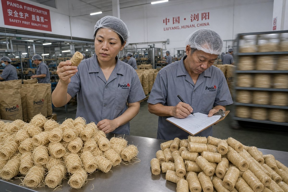
A real factory has options a trading company does not. Because we control our own production lines, we can shift capacity between color-flame products and wood fire starters when a buyer's season runs hot. But flexibility is not magic. It depends on three things being in place before the spike hits.
What makes fast adjustment possible
First, shared forecasts. When buyers send us their seasonal forecast in summer, we can pre-book wood wool, wax, and packaging materials. Raw materials are usually the longest internal lead time. If they are already staged, a repeat production run can start in days instead of weeks.
Second, staggered ordering. Instead of one giant PO, split the season into two or three tranches. Confirm the first firmly, and hold the second as a flexible commitment you finalize once early-season sell-through data arrives. This turns your forecast into a living plan.
Third, leading indicators. Demand spikes rarely come from nowhere. Falling temperatures, rising heating degree days, and surging search interest in fire-starting topics typically lead retail sales by two to three weeks. Buyers who watch these signals can trigger a reorder before shelves empty.
What to ask your supplier before the season
- How much capacity can you reserve for my SKUs during Q4?
- What is your fastest realistic turnaround on a repeat run with approved artwork?
- Can we agree on a flexible second tranche with a decision deadline?
- Will batch-to-batch quality stay consistent on a rushed run?
That last question matters. Our ISO 9001 5 process controls exist precisely so an urgent November run matches the approved sample from June. Speed without consistency just creates a different problem on your shelf. Strong supply chain optimization is a two-way effort: you share data early, and your factory converts that data into readiness.
What MOQ and Reorder Strategy Should I Use to Avoid Stockouts or Overstock?
The trade-off I discuss most with new buyers is this: order big for a lower unit cost, or order lean to protect cash. Neither extreme wins. Structure wins.
Use a base-plus-replenishment strategy: place an initial order covering 60–70% of forecast peak demand before the season, then trigger reorders using a reorder point of lead-time demand plus safety stock. Negotiate MOQs that allow a trial order first and mid-season top-ups later.

Stockout prevention and overstock avoidance pull in opposite directions. The resolution is not a bigger buffer everywhere. It is placing the right buffer at the right point in the season, and matching your MOQ structure to your forecast confidence.
Compare the three common strategies
| Strategy | How It Works | Best For | Main Risk |
|---|---|---|---|
| One big pre-season order | Buy 100%+ of forecast upfront | Long lead times, stable demand | Cash tied up; overstock if season underperforms |
| Base + replenishment | 60–70% upfront, reorder on sell-through | Most seasonal fire starter buyers | Requires supplier speed and monitoring |
| Pure just-in-time | Small frequent orders | Short domestic lead times only | Nearly impossible with ocean freight |
For imported wood fire starters, the middle path usually wins. Your initial order captures the economic order quantity 6 benefits of consolidated freight. Your replenishment tranche corrects forecast error with real data.
Set the numbers
Your reorder point is expected demand during lead time plus safety stock. If your peak-month forecast is 2,300 units, lead time is 6 weeks, and weekly peak demand is about 575 units, lead-time demand is roughly 3,450 units. Add safety stock — many small operators use a rough 20–30% buffer, though the Z × σ × √L formula is more precise when demand variability is high.
Then check your inventory turnover ratio 7 after the season. If starters sat for months, your safety stock levels were too fat. If you stocked out, they were too thin. On MOQs, talk to your factory honestly. We regularly structure flexible MOQs for trial orders, then scale volumes once a buyer's private-label line proves itself. Locking a new customer into a huge first order helps nobody — a right-sized first season builds the trust that makes year two easy.
Conclusion
Guesswork loses peak season. Clean history, seasonal indices, growth adjustment, backward lead-time planning, and a staged reorder strategy turn past sales into a confident purchase order. We help buyers run exactly this playbook every year.
Footnotes
1. Authoritative source explaining heating degree days used as a demand leading indicator. ↩︎
2. Background on advanced forecasting models mentioned as next-step techniques beyond seasonal indices. ↩︎
3. Explains the statistical safety stock concept referenced in the lead-time calculation. ↩︎
4. Defines the inventory reorder point concept central to the replenishment strategy. ↩︎
5. Official NIST resource explaining ISO 9001 quality management standards and implementation. ↩︎
6. Wikipedia background on the inventory ordering concept mentioned for consolidated freight benefits. ↩︎
7. Comprehensive Wikipedia entry defining inventory turnover ratio and its calculation. ↩︎



 English
  Spanish
  German
  French
  Arabic
  Portuguese
Join the Conversation