


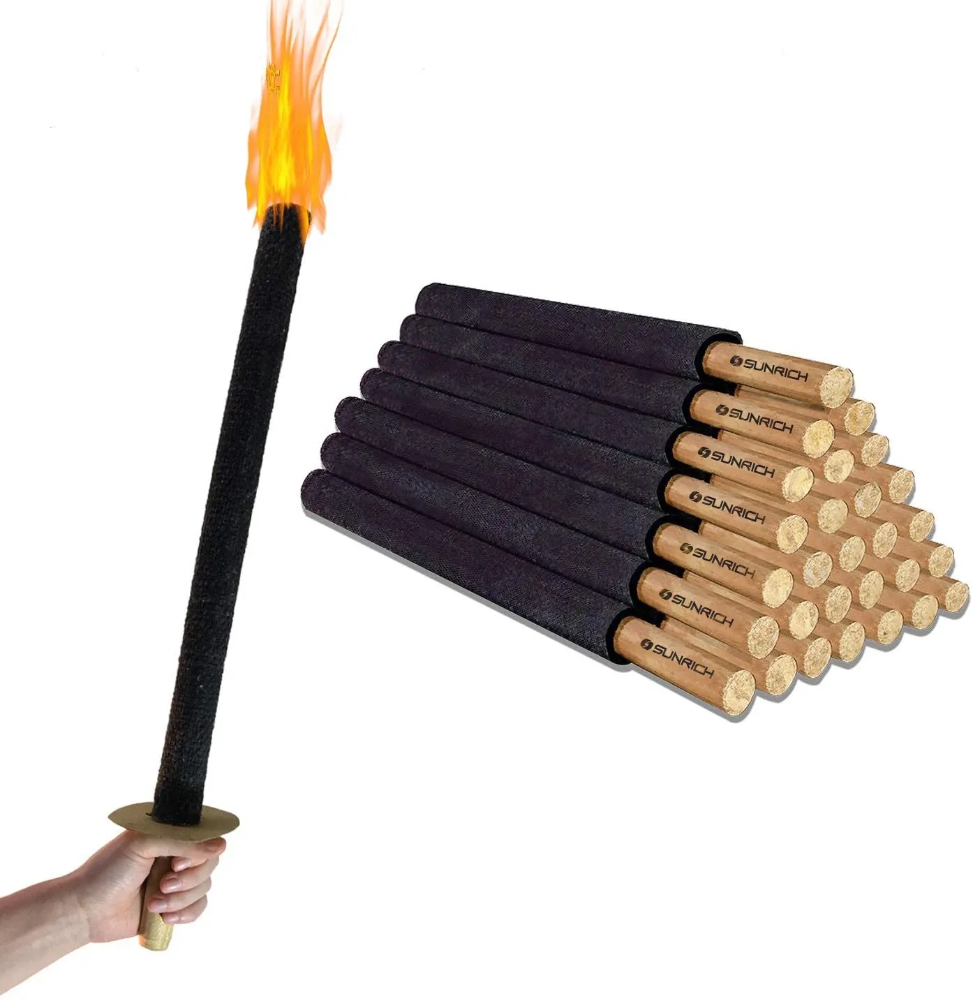




Forecasting wood fire starters purchase quantities keeps our buyers awake at night. Every spring, distributors call our factory asking us to take back pallets they over-ordered. Leftover stock ties up cash, warehouse space, and next season's budget. The fix is a simple, disciplined demand-planning workflow — and I will walk you through it.
To forecast wood fire starter purchase quantities, start with last season's monthly unit sales, apply seasonality indices, adjust for region and promotions, then order using this formula: forecast demand during lead time plus safety stock, minus on-hand and on-order inventory. Reorder in smaller waves, never one bulk buy.
That formula sounds simple. Making it work takes the right data, the right supplier terms, and the right timing. Let's break each piece down step by step.
What sales data should I track to build an accurate seasonal demand forecast for wood fire starters?
Last October, a German distributor showed me his spreadsheet: one number — total annual boxes sold. That single figure hid a 22% swing between his summer peak and his late-winter trough. Our production planning team helped him rebuild it.
Track weekly or monthly unit sell-through by SKU and channel, not annual revenue. Add at least two years of historical sales data, seasonality indices per month, inventory turnover ratio, promotion lift, and returns. Convert pack sizes into individual starter pieces so different packaging formats stay comparable.

Annual totals are the enemy of good forecasting. Wood fire starters behave like a seasonal convenience item. Demand is uneven across the year, so your data needs to capture that unevenness, not average it away. In my experience supplying fireplace distributors across the US, Germany, and the UK, the buyers who avoid season-end overstock all track the same handful of metrics.
The core data inputs, ranked by importance
| Data Input | Why It Matters | How Often to Review |
|---|---|---|
| Weekly/monthly unit sales by SKU | Reveals the true seasonal curve | Weekly in season |
| Sell-through rate per channel | Retail vs. wholesale behave differently | Weekly in season |
| Inventory turnover ratio 1 | Shows if stock is moving or sitting | Monthly |
| Pieces per pack (normalized units) | A 100-pc box ≠ a 15-pc bag | At every SKU change |
| Promotion and markdown history | Separates real demand from discount spikes | Per campaign |
| Returns and damaged stock | Corrects inflated sales figures | Monthly |
Normalize to pieces, not boxes
This point trips up more buyers than any other. One of our clients sells a 100-piece retail box through big-box channels and smaller consumer bags online. If you forecast by "boxes," a shift in pack mix will wreck your numbers. Always convert historical sales data analysis into individual starter pieces first, then translate back into boxes when you place the purchase order.
Build simple seasonality indices
Divide each month's sales by your monthly average. If December indexes at 1.4 and February at 0.7, your purchase plan should mirror that shape. Two to three years of data smooths out one-off weather anomalies. If you only have one season of history, use it — but widen your safety stock levels 2 to cover forecast error, and tighten your review cycle to weekly.
How can flexible MOQs help me test demand before committing to a full-season order?
There is a trade-off we discuss with almost every new buyer: bulk pricing looks great on a quote sheet, but a container of unsold wax-dipped wood rolls in April looks terrible on a balance sheet. Our OEM program was built around exactly this tension.
Flexible MOQs let you place a smaller trial order early in the season, measure real sell-through for four to six weeks, then scale replenishment based on actual demand. This staged approach cuts carrying costs of inventory and limits downside if the season underperforms.

The bulk-buy temptation is real. Suppliers offer discount tiers, and a full-season order at the lowest unit price feels like smart procurement. But unit price is only one cost. Carrying costs of inventory — warehousing, insurance, tied-up capital, and eventual markdowns — often erase the discount entirely when stock lingers past the season.
A staged buying plan that actually works
Here is the sequence we recommend to distributors testing our wood firestarters in a new market:
- Trial order at reduced MOQ. Cover roughly 30–40% of your forecast peak-season demand. Ship it to arrive four to six weeks before your demand curve rises.
- Measure sell-through weekly. Compare actual units sold against your forecast. Anything within 15% of plan means your model is holding.
- Place the main replenishment order. Size it using real velocity, not hope. This order should arrive just as trial stock draws down.
- Late-season top-ups only if turnover supports it. If your inventory turnover ratio slows, switch to refill-only ordering and skip the final wave.
Why we offer trial MOQs at all
Honestly, small first orders cost us efficiency on the production line. But over 17 years of exporting, we have learned that buyers who test first come back with larger, better-timed repeat orders — and they stay for years. A partner who overstocks once often disappears. Because our batch-to-batch quality control keeps mass production consistent with the first sample ISO 9001 quality standards 3, buyers can scale from a trial order without re-testing quality, which makes the staged model practical instead of theoretical.
One caution: keep trial and bulk channels separate in your forecast. A wholesaler buying 100-piece boxes behaves nothing like a consumer buying a small bag online. Forecast each channel's demand independently, then combine them at the purchase-order stage.
What lead times should I plan for with my supplier to avoid last-minute overstock or stockouts?
A UK fireplace brand once emailed us in late September asking for a full container "before the cold hits." Ocean freight 4 from Ningbo alone made that impossible. That conversation changed how we coach buyers on procurement lead time.
Plan for 30–45 days of production plus 25–40 days of ocean freight, so total procurement lead time runs 8–12 weeks to the US or Europe. Place peak-season orders by June or July, and schedule your final seasonal shipment to arrive before demand peaks — never after.

Lead time is where forecasting meets reality. Even a perfect demand forecast fails if the goods arrive after the demand window closes. From our production base in Ningbo, we ship to 30+ countries, and the calendar below reflects what actually works for a Northern Hemisphere fireplace-and-camping season.
A realistic ordering calendar for a US or EU buyer
| Timing | Action | Why |
|---|---|---|
| May–June | Finalize forecast, confirm packaging and labels | Custom private-label boxes add production time |
| June–July | Place main peak-season order | Beats the pre-holiday factory and freight crunch |
| August–September | Goods arrive; trial stock already selling | Stock lands before demand accelerates |
| October | Place one measured replenishment order | Sized from live sell-through data |
| November–December | Last shipment arrives; stop-buy after this | Anything ordered later risks arriving post-peak |
| January–February | Markdown plan activates if turnover slows | Clear stock before the spring demand cliff |
Build safety stock from lead-time variability, not gut feel
Your reorder point calculation should be: average daily demand × lead time in days, plus safety stock. Set safety stock levels from the variability of both demand and lead time. If your supplier's lead time swings between 8 and 12 weeks, that four-week spread — not a flat "add 20%" rule — should size your buffer. Peak shipping season, Chinese factory holidays, and port congestion all widen that spread, so we always flag Golden Week and Chinese New Year to our buyers months in advance.
The last-order discipline
The single most effective overstock protection is a hard "final order date." After it, you accept the small risk of a stockout in the season's last weeks rather than the large risk of carrying inventory for eight off-season months. Stockouts cost you one sale; overstock costs you margin, cash, and warehouse space until next winter.
How do regional climate and holiday patterns affect my wood fire starter purchase timing across different markets?
Shipping the same product to Brazil, Poland, and Australia taught our export team a blunt lesson: there is no single "fire starter season." Each market has its own curve, and blending them into one forecast guarantees mistiming somewhere.
Cold-climate markets peak from October through January around fireplace use and holidays, while camping-driven demand peaks in late spring and summer. Southern Hemisphere seasons invert entirely. Forecast each region separately using local heating degree days, holiday calendars, and outdoor-recreation patterns.
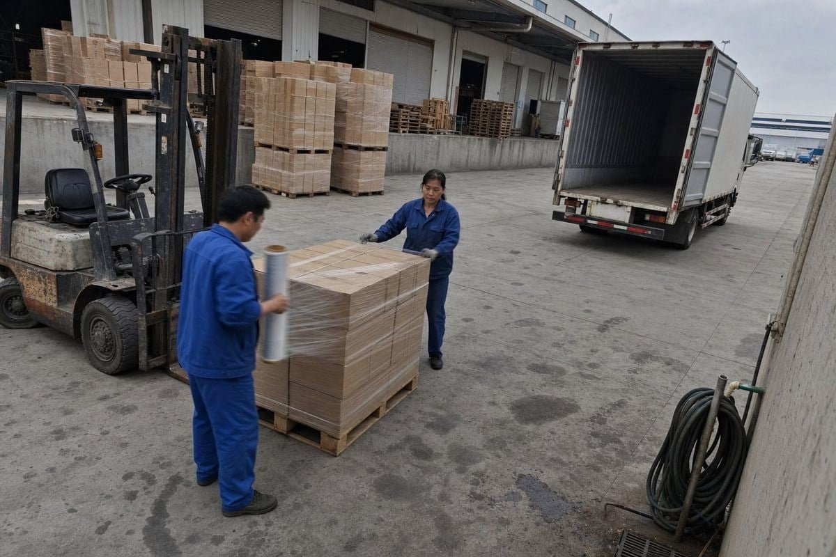
Regional demand splits along two axes: climate and use case. Fireplace and wood-stove demand follows cold weather. Camping, BBQ, and fire-pit demand follows warm weather and holidays. Many of our distributor partners serve both, which actually smooths their annual curve — if they plan each segment separately.
How major markets differ
| Market | Primary Demand Driver | Peak Window | Timing Note |
|---|---|---|---|
| US & Canada | Fireplaces + strong camping culture | Oct–Jan and May–Aug | Two peaks; North America holds a large share of global demand |
| Germany, UK, Netherlands, Poland | Wood stoves, holiday fires | Oct–Feb | Energy prices shift wood-burning demand year to year |
| Australia | Winter heating + camping | May–Aug | Inverted season; order from China by Feb–Mar |
| Brazil | Grilling and outdoor gatherings | Jun–Sep (cooler months) | BBQ culture drives steadier baseline demand |
| Middle East | Desert camping, fire pits | Nov–Mar | Winter outdoor season, opposite of intuition |
Use weather signals, not just the calendar
Heating degree days 5 are the most practical climate metric for fireplace-driven markets. A winter running 15% warmer than average means fewer burn nights, slower sell-through, and an early markdown decision — ideally in January, before the spring thaw kills demand entirely. Some sophisticated buyers go further, watching long-range forecasts for La Niña winters 6 and adjusting order volumes upward before severe cold cycles. Others correlate stock with local firewood conditions: regions with wet summers produce damper firewood, and damp wood consumes noticeably more starter material per fire.
Holidays create sharp, plannable spikes
Thanksgiving, Christmas, and New Year drive fireplace demand in the US and Europe. Memorial Day through Labor Day drives US camping demand. Because these seasonal demand fluctuations are predictable, plan promotion lift for them separately in your demand forecasting models 7 rather than letting holiday spikes distort your baseline. When we produce private-label runs for holiday gift channels, buyers lock those quantities months ahead — the display packaging and warning labels alone need lead time.
Conclusion
Season-end overstock is not bad luck. It is the predictable result of ordering annual volumes without monthly discipline. Forecast sell-through weekly, stage your orders, respect lead times, and plan regional curves separately. Do that, and your last pallet sells before the season ends — not after. Our factory has helped distributors run this playbook for over 17 years, and we are glad to help you build yours.
Footnotes
1. Defines the turnover metric buyers use to time replenishment and markdown decisions. ↩︎
2. Background on the inventory buffer concept referenced for lead-time variability. ↩︎
3. Authoritative Wikipedia entry for the standard; avoids 403 errors common on the official ISO site. ↩︎
4. WTO oversees global trade rules governing shipping and ocean freight lead times. ↩︎
5. EPA authority on the climate metric used to gauge fireplace-driven heating demand. ↩︎
6. NOAA is the authoritative source on La Niña climate cycles affecting cold-season demand. ↩︎
7. Explains the forecasting methodology underlying the article's seasonal planning approach. ↩︎



 English
  Spanish
  German
  French
  Arabic
  Portuguese
Join the Conversation